Adaboost The Original Boosting Algorithm

In this post the famous AdaBoost algoritm will be implemented in R and tested on simulated data. The post is intented to yield some intuition and understanding about what boosting is via an exercise.

What is boosting? Lets start explaining this with a nice analogy provided by the masters of boosting: Yoav Freund and Robert E. Schapire, you could imagine the horse racing-gampler being an overly intelligent gambler from Peaky Blinders:

“… A horse-racing gambler, hoping to maximize his winnings, decides to create a computer program that will accurately predict the winner of a horse race based on the usual information (number of races recently won by each horse, betting odds for each horse, etc.). To create such a program, he asks a highly successful expert gambler to explain his betting strategy. Not surprisingly, the expert is unable to articulate a grand set of rules for selecting a horse. On the other hand, when presented with the data for a specific set of races, the expert has no trouble coming up with a “rule of thumb” for that set of races (such as, “Bet on the horse that has recently won the most races” or “Bet on the horse with the most favored odds”). Although such a rule of thumb, by itself, is obviously very rough and inaccurate, it is not unreasonable to expect it to provide predictions that are at least a little bit better than random guessing. Furthermore, by repeatedly asking the expert’s opinion on different collections of races, the gambler is able to extract many rules of thumb. In order to use these rules of thumb to maximum advantage, there are two problems faced by the gambler: First, how should he choose the collections of races presented to the expert so as to extract rules of thumb from the expert that will be the most useful? Second, once he has collected many rules of thumb, how can they be combined into a single, highly accurate prediction rule? …” -Yoav Freund and Robert E. Schapire

The idea of boosting is to take these weak rules of thumbs, also called weak classifiers \(h_t\), and via a procedure, called a boosting algorithm, produce a strong classifier.

\[H_T(x)=\text{sign}\sum_{t=0}^T \alpha_t h_t(x)\]

AdaBoost was the first really succesful boosting algorithm, it has undergone a lot of empirical testing and theoretical study. If you are more interested after this post, in the theory, then I suggest you look into the book [2].

Packages

The packages that will be used in this post is the ggplot2, a package used for plotting in R, latex2exp, which is used to insert some latex code in R and pacman which has the function pacman::p_load that can be used to install and load packages,

pacman::p_load(ggplot2, latex2exp)

The pacman::p_load function can be seen as a more robust alternative to the functions require and library, which are usually used to load in packages.

Simulating data

To have complete control over the set-up for this exercise, the data for the classification problem will be simulated. First we will simulate m <- 10^5 datapoints in a circle with added noise sd<-0.13, and put the result in the dataframe circ.df, with the label -1.

theta <- runif(m, 0, 2*pi)
circ.x <- cos(theta) + rnorm(m,sd=sd)
circ.y <- sin(theta) + rnorm(m,sd=sd)
circ.df <- data.frame(label = -1, x = circ.x, y = circ.y)

Simulate m points inside the circle with added noise and put it in center.df.

center.x <- rnorm(m,sd=sd)
center.y <- rnorm(m,sd=sd)
center.df <- data.frame(label = 1, x = center.x, y = center.y)

Bind the two dataframes together row-wise with rbind and scrample the data s.t. they don’t lie in order.

df <- rbind(circ.df, center.df)
df <- df[sample(1:dim(df)[1],dim(df)[1]),]

Split it up in a training- and test- set, s.t. the model can be validated on the test-set afterwards

train <- df[1:round(dim(df)[1]/2),]
test <- df[round(dim(df)[1]/2):dim(df)[1],]
train.X <- train[,-1]
train.y <- train[,1]
test.X <- test[,-1]
test.y <- test[,1]

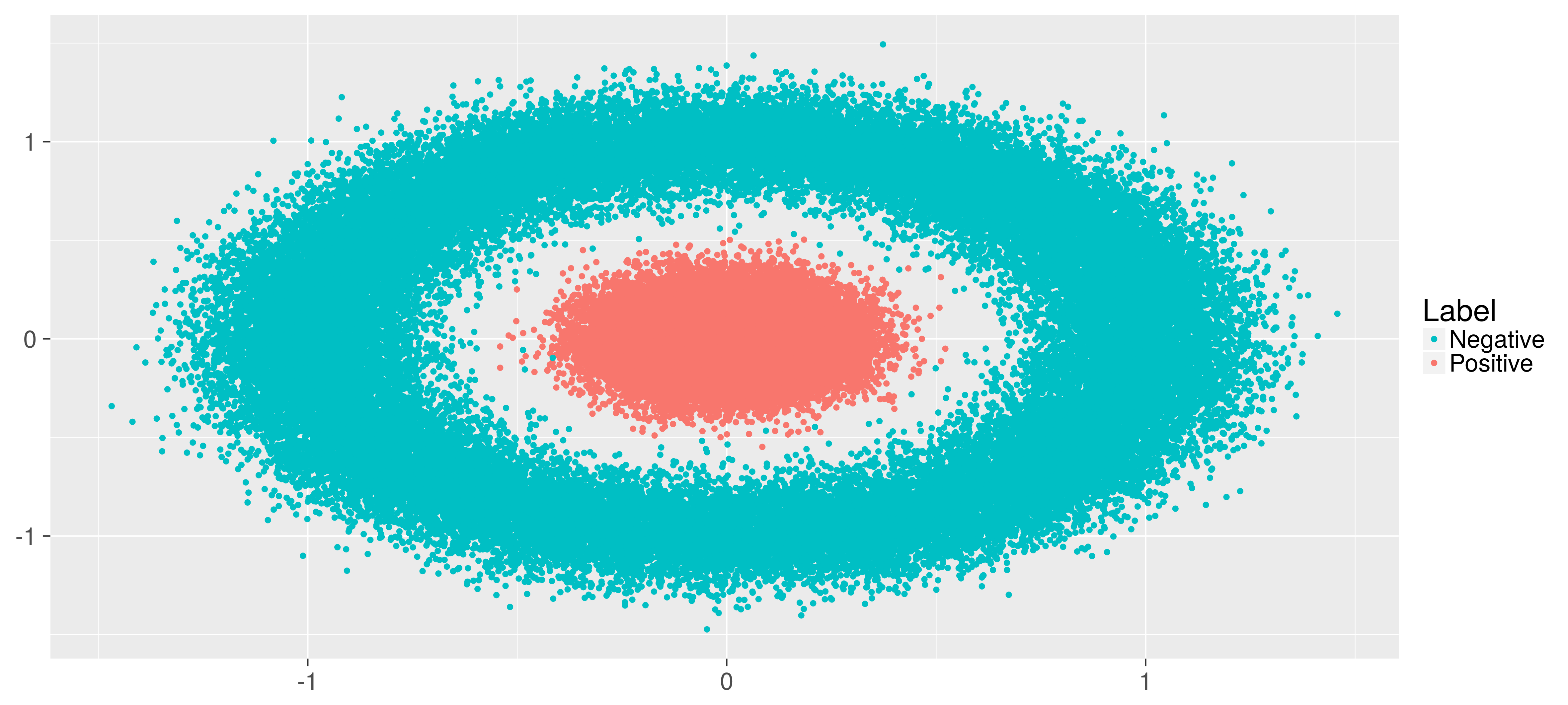
Finally plot the training data to see how it looks like. The blue points are those simulated on the circle, with label -1, and the red are the ones simulated inside the circle, label 1.

Make weak classifier

The basic component of boosting is the weak classifiers, these are the rules of thumb in the above analogy. The AdaBoost algorithm combines these to a strong classifer.

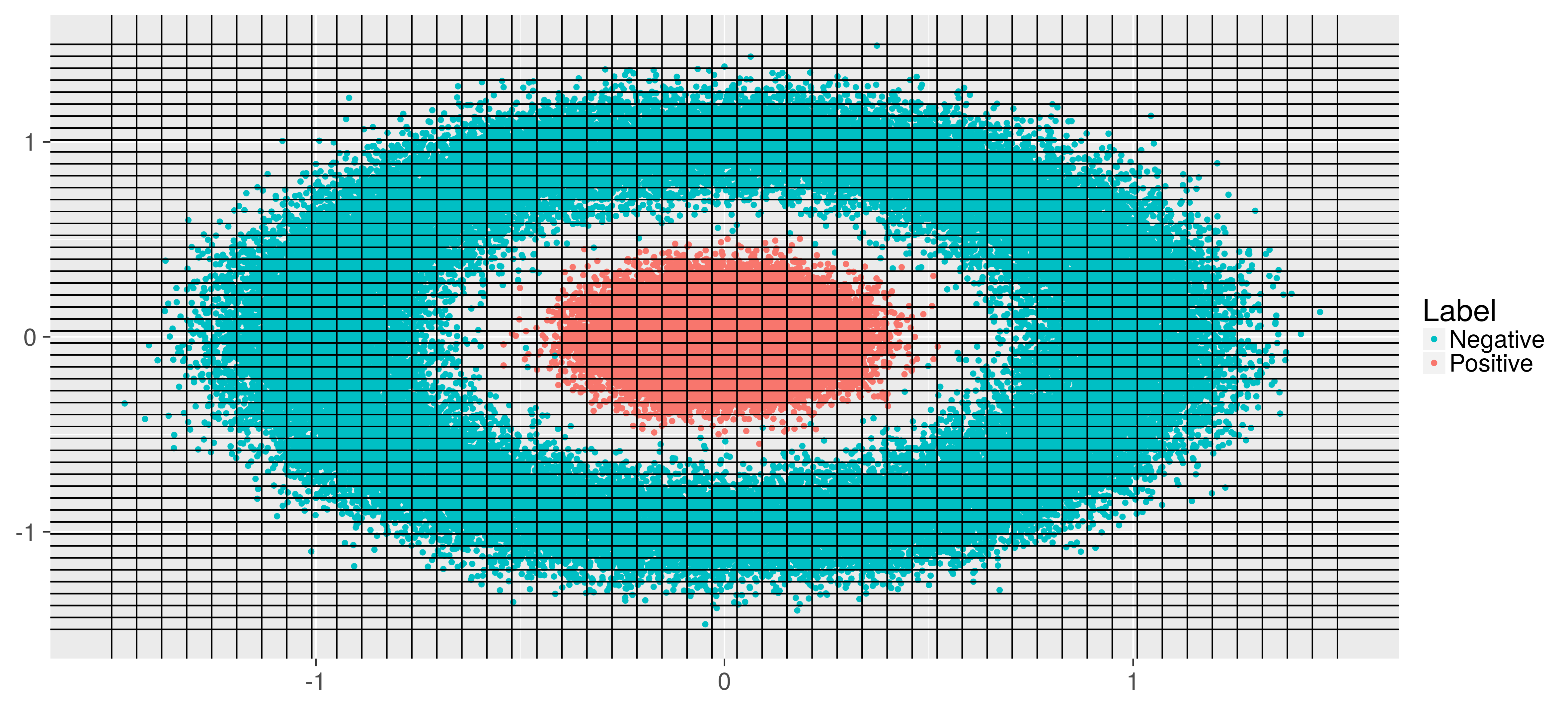
Say we have some prior knowlede about the problem and decides to construct the weak classifiers as follows: First make a finite set of classifiers, which are plotted below, for each line below (vertical and horizontal) there are two hypotheses, one which is positive when points is on one side of the line, and one which is positive when point is on the other side. The classifier selected is then the one which minimizes the weigthed error:

\[e_t=\sum_{i=0}^{2m} w_i 1\{h_t(x_i)\neq y_i\}\]

In practice the weak classifiers are often simple decision trees, could be stumps: Trees with only one split. But in general one could try out the AdaBoost with almost any procedure in which one can weigh the error.

The AdaBoost algorithm

The algorithm keeps some quantities throughout a loop. These are here implemented below.

w <- rep(1/nrow(train.X),nrow(train.X))
H <- list()
alphas <- list()

The w denotes the weights presented above. These can be viewed as a probability distribution held over, in each round t of AdaBoost, the observations, and initialized as uniform. This distribution is used to fit a weak classifier h_t in each iteration, and to get a weighted accuracy e_t.

Two additional quantities are also keept throughout the loops. The training error and test error:

train_err <- c()
test_err <- c()

these will be used for evaluation of the algorithm afterwards.

for(t in 1:T_){

  res <- fit(train.X, train.y, H.space, w)

  e_t <- res[[1]]

  h_t <- res[[2]]

  alpha_t <- 1/2 * log((1-e_t)/e_t)

  Z_t <-  2*sqrt(e_t*(1-e_t))

  w <- w * exp(-alpha_t*train.y*predict(train.X,list(h_t),1)) / Z_t

  alphas[[t]] <- alpha_t
  H[[t]] <- h_t


  train_err <- c(train_err, mean(predict(train.X,H,alphas) != train.y))
  test_err <- c(test_err, mean(predict(test.X,H,alphas) != test.y))
}

The weighted accuracy e_t is used to weigh the new weak hypothesis in the final ensemble by alpha_t, weighing them s.t. they greedly contributes the most to the ensemble in terms of in-sample error. This can also intuitively be inferred by a plot of the functional dependency between these two quantities

At the end of each iteration the distribution w is updated, putting more weight to incorrectly classified observations w * exp(-alpha_t*train.y*predict(train.X,list(h_t),1)). The Z_t is used for normalization of the weights to a probability distribution.

Running the algorithm

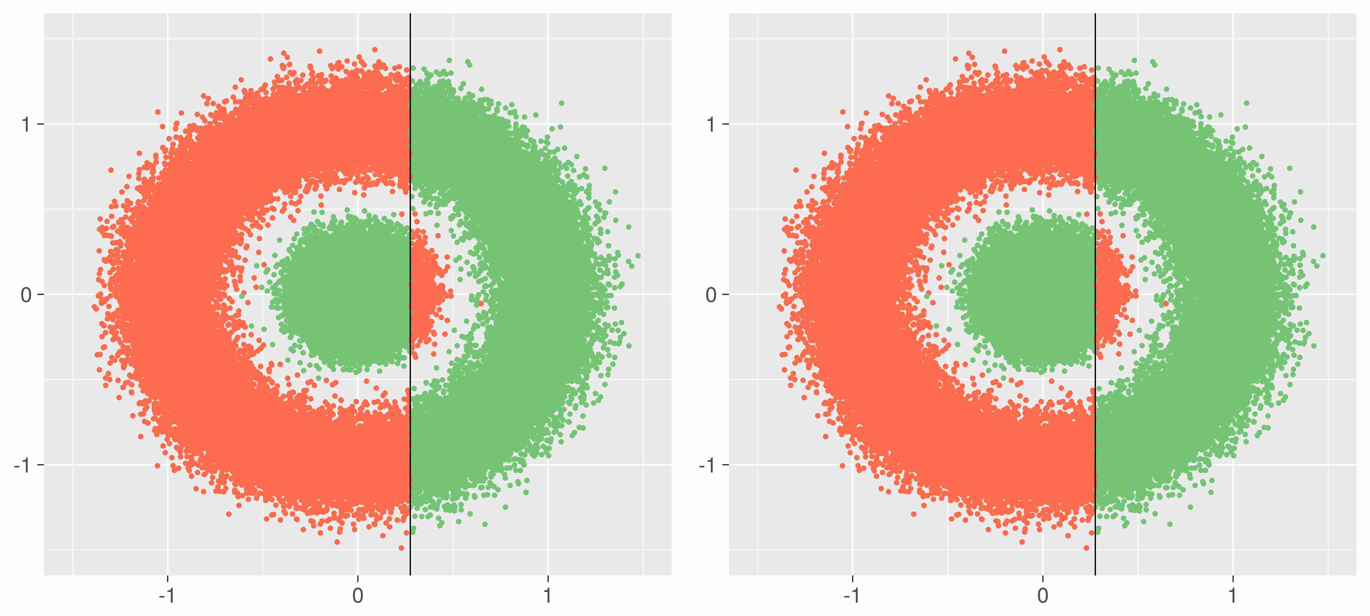
Below one sees how the algorithm combines the weak classifiers. To the left one sees the combined classifier at iteration t and to the right the hypothesis fitted at iteration t of AdaBoost. Observations marked green is classified correctly by the given hypothesis and observations marked red are classified incorrectly. One observes how AdaBoost zooms in on the observations which is hard to classify, in the last iterations: Those on the inside of the circle. AdaBoost is also used in the outlier detection because of this property.

One also observes the algorithm sometimes chooses a hypothesis to the far right classifying all observations as the same, which makes sense when the majority of the observations, in the weighted error at the given iteration, is of that label, as seen in iteration 3, it does seem to make sense in the ensemble to add this seemingly useless classifier.

Result on the test set

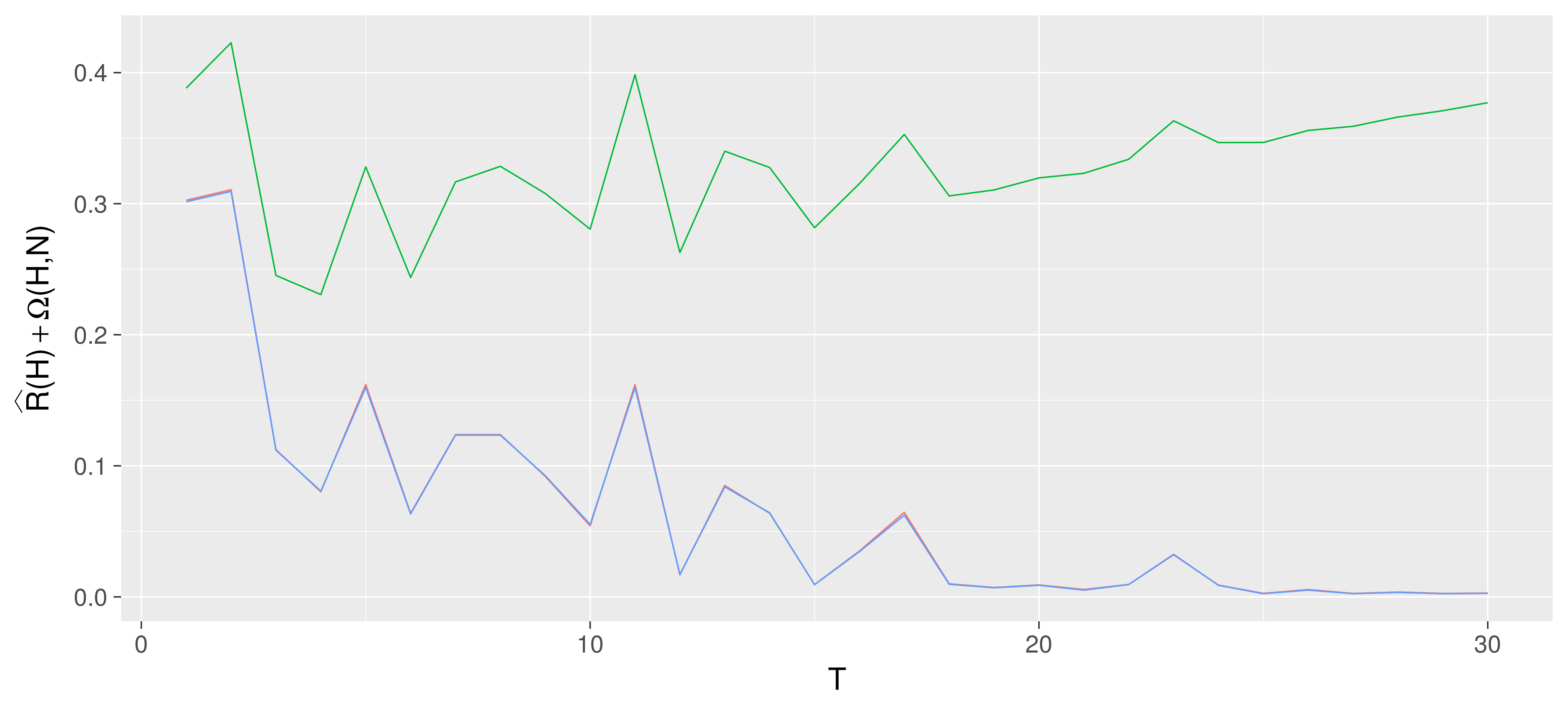
Below one sees the training- (blue) and test- (red) error, which seems to be almost identical in this example. The green line is plot off a probably almost correct (PAC) learning bound: A bound on how bad an algorithm can perform under some rather general statistical assumptions, with a given probability, hence probably almost. The below green line is a plot of this bound: Out-of-sample error is below this line with 95% probability. The bound seems to predict a fast overfitting as a function of the number of trees, i.e. one observes that the bound increases very fast as a function of the number of trees in the ensemble, it cannot bound the generalization error.

But as seen in the plotted training- and test-error, red and blue, it seems to be benificial to run AdaBoost in more rounds than indicated by the bound, which is also the case in practical applications.

One interesting aspect about these bounds on generalization performance from a practical point of view, is that they can often be decomposed into two terms,

\[R(H) \leq \hat{R}(H)+\Omega(H)\]

Where \(R(H)\) is the true generalization error, \((H)\) is the in-sample loss, which decreases as a function of complexity, here being the number of trees in the ensemble, and \((H)\) is a complexity term, which increases as a complexity increases, here it increases as the number of trees grows. Such bounds, found many places in theory, indicates a trade-off between in-sample fit and complexity, a phenomenon also sees in practice.

Conclusion

This post touched the surface of some components of AdaBoost, and hopefully woke some interest into these types of algorithms.

References

[1] Yoav Freund and Robert E. Schapire, A Short Introduction to Boosting. Journal of Japanese Society for Artificial Intelligence, 1999

[2] Yoav Freund and Robert E. Schapire, Boosting: Foundations and Algorithms. The MIT Press, 2012

Comments

Feel free to comment here below. A Github account is required.