XGBoost

In this post we will go through an example application of the XGBoost algorithm using data from a competition on the crowdsourced machine learning homepage Kaggle. We will show some of the model diagnostics one can make with XGBoost. One of these being the partial dependence plot, which is a general technique for analyzing black box methods like XGBoost.

Data

We will use the data from the Kaggle competition: “House Prices: Advanced Regression Techniques”, you can download it from this link: Data. We will only use the train.csv file. Remember to set the csv on your current working directory in R, you can use the setwd(directory) function in R, to set the working directory to the directory that contains the data.

Packages

We will use the readr-package which we will use to read in the csv-file containing the data. The xgboost-package which contains the implementation of XGBoost in R. The Matrix-package which will be used to construct a sparse model matrix that we will feed to the XGBoost algorithm. The DiagrammeR-package and igraph-package which XGBoost uses for plotting and one of these plotting tools depend upon the package Ckmeans.1d.dp. The ggplot2-package for plotting and the gridExtra-package for plotting a grid in ggplot2.

And finally the dplyr package, this package is purely a convinience package for data-manipulation in R, it contains the pipe operator %>% which takes the output of the function to the left and feeds it to the first argument of the function to the right. Besides being very intuitive it also makes your code more readable.

pacman::p_load(readr, xgboost, Matrix, igraph, DiagrammeR, Ckmeans.1d.dp, ggplot, gridExtra, dplyr)

Read data and formatting

Lets read in the data, put it in a data.frame and change character columns to factor columns, awesomely done using dplyr.

train <- read_csv("train.csv") %>% data.frame() %>% mutate_if(is.character, factor)

Now lets prepare the data for the algorithm. First lets construct a matrix with the factors expanded using one-hot-encoding, and lets do expand it to a sparse matrix instead of a regular matrix by using sparse.model.matrix from the Matrix-package, this is better for memory consumption if it were a larger dataset.

The model.matrix function in R is usually used for linear regression, R uses it to expand factors and interactions in the model formula out into dummies using the contrasts argument, the sparse.model.matrix function does the same thing but outputs a sparse matrix. Here we will use it for one-hot-encoding of the factors.

xg.data <-
  sparse.model.matrix(~ . -1,
                    model.frame(train[,-which(names(train) %in% "SalePrice")],na.action = na.pass),
                    contrasts.arg = lapply(train[,sapply(train,is.factor)], contrasts, contrasts=FALSE))

Now we will put it in a data format for XGBoost.

xg.labelledData =xgb.DMatrix(xg.data, label=train$SalePrice)

The XGBoost model

This section is intended to give a super short intuitive introduction to XGBoost from a more mathematical point of view.

The XGBoost model is a boosting model, it is a more advanced version of a normal gradient boosting model, which is fairly easy to understand. In normal gradient boosting the objective is to minimize the loss function:

\[\mathcal{L}(F) := \frac{1}{N} \sum_{i=1}^{N} L(F(x_i),y_i)\]

For the purpose of this minimization one is only interested in \(F\) evaluated at \(F(x_1),...,F(x_N)\) which one can regard as \(N\) real variables: \[f_i:=F(x_i)\in\mathbb{R}\] Viewed this way the goal is now to minimize: \(\mathcal{L}(f_1,...,f_N) = \frac{1}{N} \sum_{i=1}^{N} L(f_i,y_i)\). So one observes that \(\mathcal{L}\) can be thought of as a real-valued function defined on \(\mathbb{R}^N\), one which can be minimized by applying gradient descent i.e. initialize \(F=(f_1,...,f_N)'=0\in\mathbb{R}^N\) and update using \[ F \gets F - \eta \nabla \mathcal{L}(F)\] Where \(\nabla\mathcal{L}:=(\frac{\partial\mathcal{L}}{\partial f_1},...,\frac{\partial\mathcal{L}}{\partial f_N})'\) is the gradient evaluated in the current in-sample predictions \(F=(f_1,...,f_N)'\).

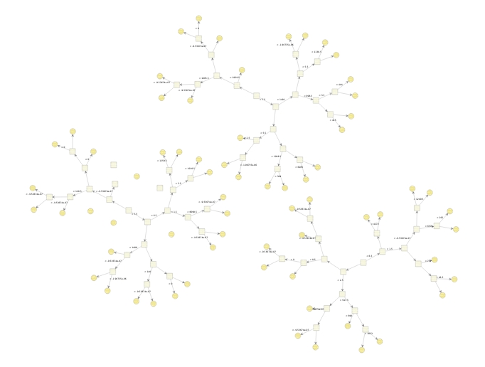
This procedure does not specify any meaningful prediction out-of-sample, because one is only minimizing \(\mathcal{L}\) with respect to \((f_1,...,f_N)'=(F(x_1),...,F(x_N))'\), so this procedure only yields meaningful predictions on the training points i.e. the predictions \(F(x_1),...,F(x_N)\) for the training points \(x_1,...,x_N\). To yield meaningful prediction for inputs which is not \(x_1,...,x_N\) one imposes the restriction that each update must come from a class of base functions: \(\mathcal{H}\). One can now initialize \(F=0\in\mathbb{R}\) and use the update rule \[F \gets F - \eta h,\quad h\in\mathcal{H}\] in each iteration of this analog of gradient descent to functional space. The \(h\) is chosen to be the function closest to the gradient \(\nabla\mathcal{L}\) with respect to the euclidian norm (the \(L^2\) norm). Each of these base functions is then added to \(F\) in each iteration like the vectors is in gradient descent, such that one ends up with a final classifier that consists of a sum of these base functions: \(F=\sum_{t=1}^T h_t\). The base functions \(h_t\) most used with XGBoost is simple decision trees, but linear functions are also available. Three of such trees from the application in this article are plotted below.

XGBoost utilizes the same idea as normal gradient boosting but more like an analog of the Newton-Raphson method in functional space and with extra regularizations methods.

In XGBoost the regularized loss funtion is minimized:

\[ L(F_T)=\sum_{i=1}^{N}L[y_i,F_T(x_i)]+\sum_{t=1}^{T}\Omega(h_t), \quad F_T(x)=\sum_{t=1}^{T}h_t(x) \]

Where the extra sum over \(\Omega(h_t)\) is regularization applied to each tree. Assume that a given tree \(h_t\) has \(J_t\) terminal nodes and weights \(w_{j,t}\) in each leaf node. Then this regularization can be expressed as:

\[ \Omega(h_t) = \gamma J_t + \frac{1}{2}\lambda\sum_{j=1}^{J_t}w_{j,t}^2 + \alpha \sum_{j=1}^{J_t} \vert w_{j,t}\vert \]

From this one sees that the \(\gamma\) work as a minimal loss reduction required to make a new split in a terminal node, in an arbitrary iteration of the algorithm. The sums \(\alpha\sum_{j=1}^{J_t} \vert w_{j,t}\vert\) and \(\frac{1}{2}\lambda\sum_{j=1}^{J_t}w_{j,t}^2\) is over the weights in the leaf nodes \(w_{j,t}\) in tree \(t\)’th tree. It is \(L^1\) and \(L^2\) regularization over the weights in the leaf nodes for the \(t\)’th tree.

Besides these regularizations XGBoost also gives one the opportunity to use subsample a fraction of the dataset in each iteration, analogous to stochastic gradient descent, and to use a subsample of the columns in each iteration, like a Random Forest.

If you want to read about it I recommend you read this Chen and Guestrin [2016] article from the guys who made XGBoost, I can’t say I understand the implementation they describe in the article but this is also a great part of XGboosts succes, besides the mathematical model.

Model tuning and Validation

XGBoost consistst of a lot of parameters. The ones I have used most succesfully for regression problems are listed below, many of them with their default value. To see a list of them all go to XGBoost parameters. Besides these I also highly recommend you test the scale_pos_weight parameter if you have an imbalanced classification problem.

param <- list("booster"             = "gbtree", # specifying that the basis functions are regression trees
              "eta"                 = 0.05,     # specifying the learning rate 0<eta<1
              "gamma"               = 50,       # specifying loss for extra leaf node
              "max_depth"           = 5,        # maximum depth of tree
              "alpha"               = 0,        # L1 regularization
              "lambda"              = 1,        # L2 regularization
              "subsample"           = 0.5,      # how much of the data is used in subsampling for a new iteration(rows)
              "colsample_bytree"    = 0.8       # how much of the data is used in subsampling for a new iteration(collumns)
)

Now you can ask yourself: What to do with all these fucking parameters? Answer: Validate the model for different values of the parameters, each in a routine that gives you an approximation for generalization performance, i.e. approximates how well the algorithm will perform on new unseen data like cross-validation for stationary data or a backtest for financial data, or another routine for the given problem. Most commonly each parameter is tested in a grid search, random search or by Bayesian search. In my experience the random search works very well and is easily implemented, when implemented you can just start it, and let it run over the weekend, and then analyze the results Monday when you get back to work.

One of the routines mentioned above are implemented in the xgboost package, a cross-validation, and implemented in R below.

cvData <- xgb.cv(params = param,
                 xg.labelledData,
                 nrounds = 2000,
                 verbose = TRUE,
                 nfold = 3,
                 metrics = c("mae"))

Eventhough it is already implemented I recommend, if you have the time, that you instead make your own grid-search or other routine, s.t. you know that all the algorithms you are validating are compared consistently, and in a routine you believe approximates the generalization error.

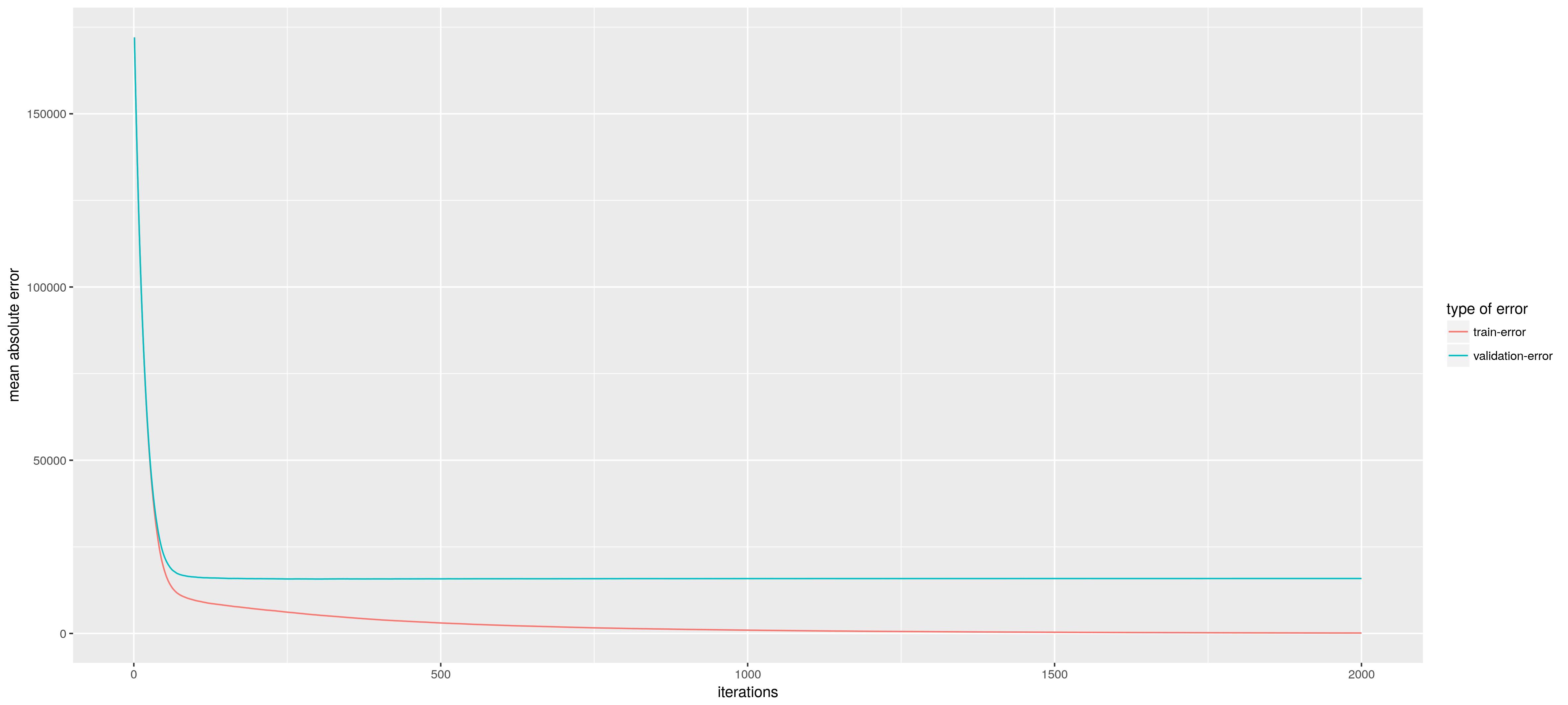
But for this post we will just use the above routine. As a output of the routine we can plot the validation error (the estimated generalization error from the cross-validation routine) together with the training error. We see that the model starts to overfit when we get more and more trees (the difference between the validation error and training error increases). But the minimum validation error is at 2000 trees so lets use that.

Now we train our model using the below code.

bst <- xgboost(params = param,
              xg.labelledData,
              nrounds = 2000,
              verbose = TRUE
)

Model inspection

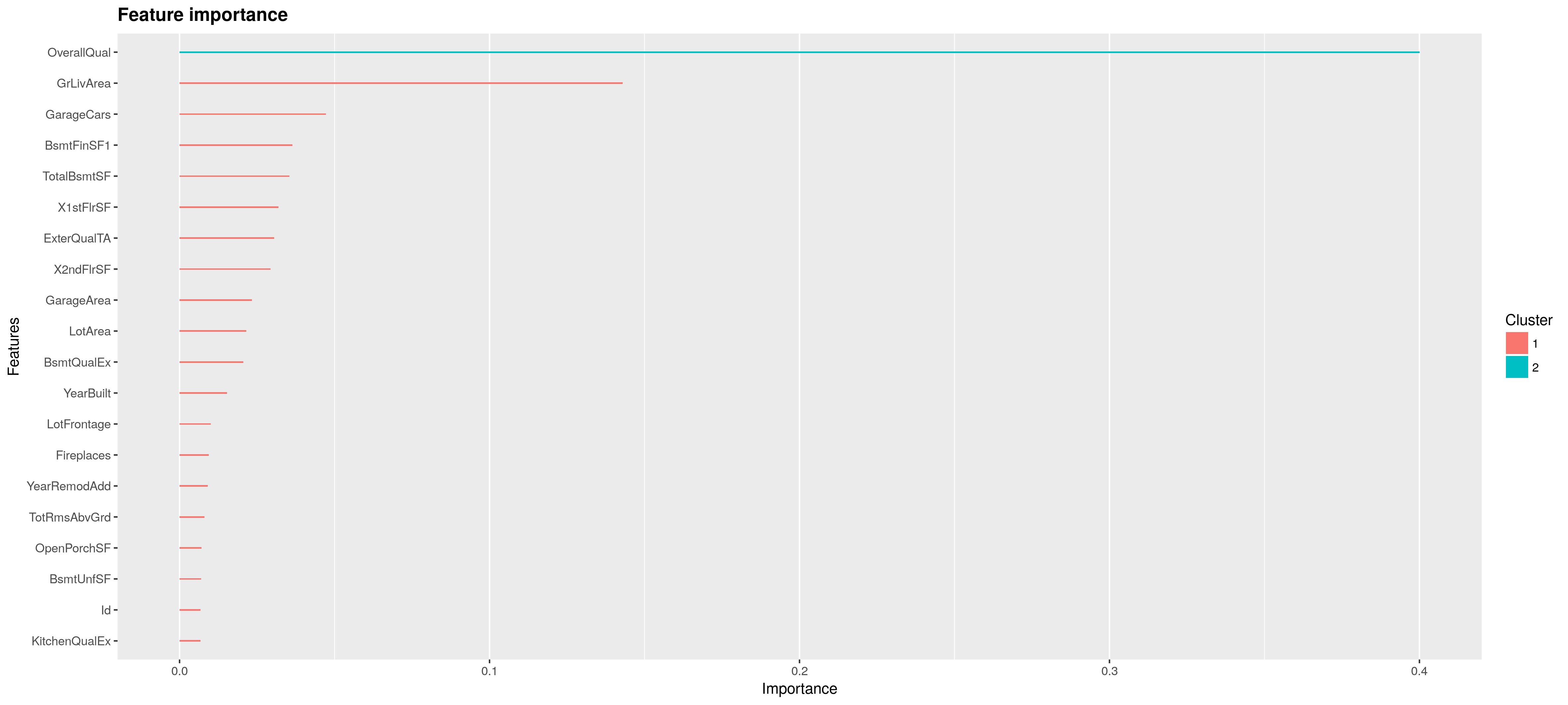
First we will plot the feature importance. Feature importance is calculated by summing over the internal nodes in the tree. In each of these nodes one of the features is applied to split the constant region in two subregions. The way this split is chosen is by the maximum improvement in loss over the constant fit in the region. Feature importance is now the sum over improvement in loss over the internal nodes for a given feature averaged over all the trees in the sum \(\sum_{t=1}^T h_t\).

importance_matrix = xgb.importance(names, model = bst)
xgb.ggplot.importance(importance_matrix, top_n = 20, n_clusters = c(1, 2))

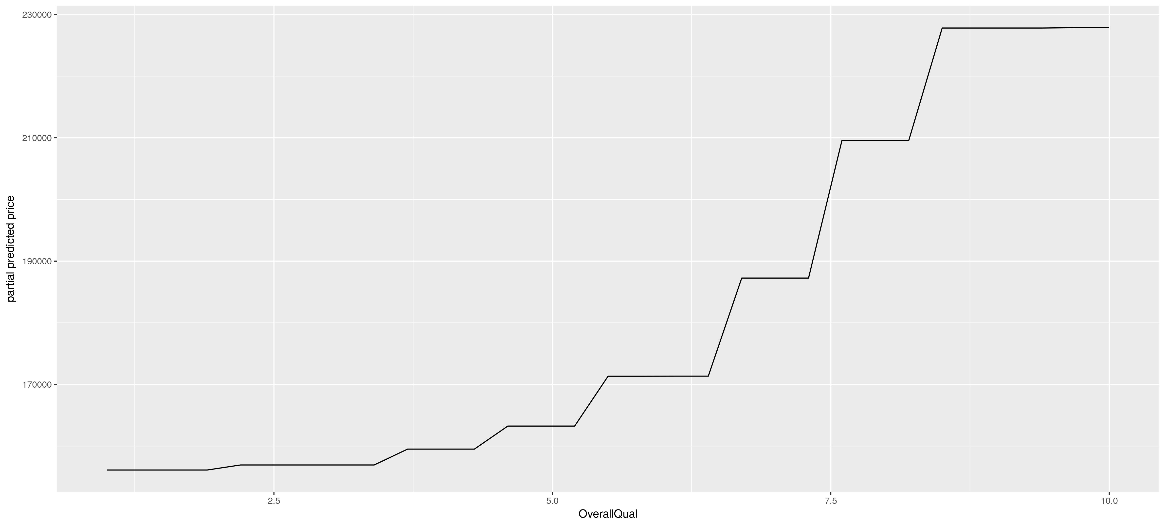
After one has identified the most important variables in the model, it is often of interest to understand the dependence of the prediction on the joint feature values. A plot of the prediction as a function of its inputs is however restricted to a functional relationship with just two inputs (\(d\leq 2\)), a 3-d plot. If one wishes to plot a model with more inputs than two one has to get creative. A smart alternative is to approximate the prediction as a function of a subset of the inputs, s.t. partial effects can be plotted in a 2-d or 3-d plot in a model with more than two inputs. This is what one does in partial dependence plots. Below is an example of such a plot, which yield a plausible partial effect of an increase in OverallQual of the house, for this model.

Mathematically you can see a partial dependence plot like it like this: Assume \(X_S\) is the partial random variables (a random vector) you wish to compute the partial effects of, you then just “average out” the other variables, the \(X_C\) random variables, using the observed values \(x_{Ci}\), which gives you the below. \[ \tilde{F}_S(X_S)=\frac{1}{N}\sum_{i=1}^{N}F(X_S,x_{iC})\] Below you see the code how to do this in R.

# make partial predictions
for(grid_i in grid){
  # constructing temporary data-frame
  train_tmp <- train
  train_tmp[,mostImpFeat] <- rep(1,dim(train_tmp)[1]) * grid_i

  # names of the regressors and the one-hot encoded factors
  xgb.train_tmp <- sparse.model.matrix(~ . -1,
                                       model.frame(train_tmp[,-which(names(train_tmp) %in% "SalePrice")],na.action = na.pass),
                                       contrasts.arg = lapply(train_tmp[,sapply(train_tmp,is.factor)], contrasts, contrasts=FALSE))

  partialPredictions <- c(partialPredictions, mean(predict(bst, newdata = xgb.train_tmp)))
}

This estimate can be heavy in calculation if the dataset is big, an easy fix is just to approximate it using a subsample of the observed sample, which still approximates the same partial relationship. It should be noted that this approximation method is not restricted to weighted sums of trees, but can be applied to any “Black Box” models. ## Conclusion This post introduced the XGBoost algorithm, which is used a lot on the Kaggle platform and in practice. It also introduced some model diagnostics for XGBoost, one of these being the partial dependence plot which is a nice general method to vizualize the effects of a black-box method in a 1D- or 2D-plot.

References

[1] Tianqi Chen and Carlos Guestrin. XGBoost: A Scalable Tree Boosting System. Discovery and Data Mining - KDD ’16, 785-794, 2016.

[2] Github Repo

Comments

Feel free to comment here below. A Github account is required.